Uncover Cell-Cell Interactions in scRNA-seq

Setup the Matchmaker Object

For this tutorial, we will be analyzing the human decidua single cell RNA-seq dataset from Vento-tormo et al. 2018 Nature. There are 64,734 single cells that were generated using 10X Genomics. The raw data can be found here. We will be using the CellPhoneDB ligands-receptors interaction repository.

A fraction of this data containing 947 ligand and receptor genes and 3000 cells (726 EVT, 953 dS2, 788 dNK1, and 533 dM1) is included in the scMatchmaker package called decidua and the corresponding metadata containing cell type annotations called decidua.annotation. This data has been normalized in logTPM (log-transformed transcripts per million), and it is recommended to start with normalized data. The Normalization function can be used to normalize raw scRNA-seq counts. It provides widely used logTPM normalization, as well as cosine normalization used in Haghverdi et al. 2018 Nature Biotechnology.

Then we load a CellPhoneDB database included in the package called cellphonedb. Alternatively, we can use LoadCellPhoneDB function to load the CellPhoneDB database either locally or from their website.

You can check the Matchmaker object structure and slot information by typing ?'Matchmaker-class'.

# Install scMatchmaker from CRAN.
if (!requireNamespace("scMatchmaker", quietly = TRUE))
    install.packages("scMatchmaker")

# Load scMatchmaker.
library(scMatchmaker)

# Load the CellPhoneDB interaction database from URLs. 
# This step is optional when using scMatchmaker's preloaded database.
interaction.url = "https://raw.githubusercontent.com/Teichlab/cellphonedb-data/master/data/interaction_input.csv"
gene.url = "https://raw.githubusercontent.com/Teichlab/cellphonedb-data/master/data/gene_input.csv"
complex.url = "https://raw.githubusercontent.com/Teichlab/cellphonedb-data/master/data/complex_input.csv" 

interaction.data <- LoadCellPhoneDB(
  interaction_input = interaction.url,
  gene_input = gene.url,
  complex_input = complex.url,
  gene.symbol = "gene_name", url = TRUE)

# Initialize Matchmaker object with scMatchmaker preloaded cellphonedb database.
# Missing ligands and receptors will be added with zeros, this step is useful when calculating protein interaction complex later.
decidua.interaction <- Screening(data = decidua, annotation = decidua.annotation[,"annotation", drop = FALSE], interaction = cellphonedb, project_name = "Decidua")
decidua.interaction
## Decidua Matchmaker object: 
## 1574 interaction pairs across 3000 cells. 
## 0 ligand-recptor pairs across 0 cell-cell interactions calculated.

What does the data look like?

# Let's look at the some example ligand and receptor genes in the first twenty cells.
decidua[c("EGFR","TGFB1","EGF"), 1:20]
## 3 x 20 sparse Matrix of class "dgCMatrix"
##                                                                                                                               
## EGFR  . .        . . .         . . .         . .         . .         .       . .        .        .        . .         .       
## TGFB1 . 1.131673 . . 0.6504162 . . 0.9582769 . 0.7757068 . 0.9077957 1.07289 . 1.122225 1.407436 1.318945 . 0.6545622 1.395667
## EGF   . .        . . .         . . .         . .         . .         .       . .        .        .        . .         .

The dots . in the decidua dataset count matrix represent 0's (no UMI). Because scRNA-seq data contains lots of 0's, Matchmaker uses this sparse matrix notation to store data, interaction strength and p values matrices to save memory. However, if there are not many zero entries, sparse matrix is no longer efficient to save memory. Matchmaker controls for this by the zero_percent parameter. The default is 0.7, that is, when the non-zero entries is above 70% the data will be saved as sparse matrix,

# Let's look at the first six rows of the corresponding metadata.
head(x = decidua.annotation)
##                             Fetus location final_cluster annotation
## FCA7196224_TCACAAGCAGTTCATG    D9  Decidua             7        dM1
## FCA7167223_AATCCAGTCACGCATA    D6  Decidua             7        dM1
## FCA7167223_GGACAGAAGTCGATAA    D6  Decidua             7        dM1
## FCA7196224_TATCTCAGTTCCCGAG    D9  Decidua             7        dM1
## FCA7196224_GTGCATATCCAATGGT    D9  Decidua             7        dM1
## FCA7167221_CGAATGTAGACCACGA    D7  Decidua             7        dM1

# Let's look at the first six rows of the CellPhoneDB interactions loaded from URLs.
head(x = interaction.data)
##   genename_a genename_b id_cp_interaction partner_a partner_b protein_name_a protein_name_b annotation_strategy         source subunit_a_1
## 1       ACE2       GHRL   CPI-SS085C150CE    Q9BYF1    Q9UBU3     ACE2_HUMAN     GHRL_HUMAN                 I2D                       <NA>
## 2      ACKR1      CCL17   CPI-SS0974EB232    Q16570    Q92583    ACKR1_HUMAN    CCL17_HUMAN                 I2D                       <NA>
## 3      ACKR2       CCL2   CPI-SS03165AD8C    O00590    P13500    ACKR2_HUMAN     CCL2_HUMAN             curated PMID: 24218476        <NA>
## 4      ACKR2       CCL3   CPI-SS04318D03E    O00590    P10147    ACKR2_HUMAN     CCL3_HUMAN             curated PMID: 24218476        <NA>
## 5      ACKR2      CCL14   CPI-SS045A5FC60    O00590    Q16627    ACKR2_HUMAN    CCL14_HUMAN             curated PMID: 24218476        <NA>
## 6      ACKR2      CCL13   CPI-SS06B0861F1    O00590    Q99616    ACKR2_HUMAN    CCL13_HUMAN             curated PMID: 24218476        <NA>
##   subunit_a_2 subunit_a_3 subunit_b_1 subunit_b_2 subunit_b_3
## 1        <NA>        <NA>        <NA>        <NA>        <NA>
## 2        <NA>        <NA>        <NA>        <NA>        <NA>
## 3        <NA>        <NA>        <NA>        <NA>        <NA>
## 4        <NA>        <NA>        <NA>        <NA>        <NA>
## 5        <NA>        <NA>        <NA>        <NA>        <NA>
## 6        <NA>        <NA>        <NA>        <NA>        <NA>

# Let's look at the first six rows of the preloaded CellPhoneDB interaction list.
head(x = cellphonedb)
##   genename_a genename_b id_cp_interaction partner_a partner_b protein_name_a protein_name_b annotation_strategy         source subunit_a_1
## 1       ACE2       GHRL   CPI-SS085C150CE    Q9BYF1    Q9UBU3     ACE2_HUMAN     GHRL_HUMAN                 I2D                       <NA>
## 2      ACKR1      CCL17   CPI-SS0974EB232    Q16570    Q92583    ACKR1_HUMAN    CCL17_HUMAN                 I2D                       <NA>
## 3      ACKR2       CCL2   CPI-SS03165AD8C    O00590    P13500    ACKR2_HUMAN     CCL2_HUMAN             curated PMID: 24218476        <NA>
## 4      ACKR2       CCL3   CPI-SS04318D03E    O00590    P10147    ACKR2_HUMAN     CCL3_HUMAN             curated PMID: 24218476        <NA>
## 5      ACKR2      CCL14   CPI-SS045A5FC60    O00590    Q16627    ACKR2_HUMAN    CCL14_HUMAN             curated PMID: 24218476        <NA>
## 6      ACKR2      CCL13   CPI-SS06B0861F1    O00590    Q99616    ACKR2_HUMAN    CCL13_HUMAN             curated PMID: 24218476        <NA>
##   subunit_a_2 subunit_a_3 subunit_b_1 subunit_b_2 subunit_b_3
## 1        <NA>        <NA>        <NA>        <NA>        <NA>
## 2        <NA>        <NA>        <NA>        <NA>        <NA>
## 3        <NA>        <NA>        <NA>        <NA>        <NA>
## 4        <NA>        <NA>        <NA>        <NA>        <NA>
## 5        <NA>        <NA>        <NA>        <NA>        <NA>
## 6        <NA>        <NA>        <NA>        <NA>        <NA>

Identify Cell-Cell Interactions with Matchmaking

Before we search for cell-cell interactions, we can optionally downsample the data with Sketching function to reduce the number of cells which may speed up the computation time.

There are two methods to perform downsampling:
- Downsample proportionally to the cell type frequencies (downsampling = TRUE). The actual downsampling size may vary slightly due to rounding effects.
- Geometric Sketching by Hie et al. 2019 Cell Systems using the input data (downsampling = FALSE).

# Downsampling the number of cells to 1000.
decidua.interaction <- Sketching(object = decidua.interaction, size = 1000, downsampling = TRUE)
decidua.interaction
## Decidua Matchmaker object: 
## 1574 interaction pairs across 1001 cells. 
## 0 ligand-recptor pairs across 0 cell-cell interactions calculated.

Which cells are being "sketched"?

# Show the frist six downsampled cell IDs.
head(x = decidua.interaction@misc$sketch_id)
## [1] 129 509 471 299 270 187

The Matchmaking function is the workhorse that calculates the interaction strengths and p values. It first calculates the interaction strengths using either a base model or an Earth Mover's Distance (EMD) adjusted model (see below). Then it randomly permutes the cell type identities for a number of times (usually 100-1000), and calculates a null distribution for each interacting pairs similar to the CellPhoneDB Python Package. This null distribution will serve as a nonparametric tests to select the significant interactions.

Matchmaking will return two interaction matrices in Matchmaker object:
- @strength stores the relative interaction strength.
- @pvalue stores the p values for each interactions.

The rows represent cell-cell interacting pairs (dM1|DC1 stands for interaction between dM1 and DC1 cell types) and the columns represent ligand-receptor pairs (i.e. ACE2_GHRL stands for interaction between ACE2 and GHRL genes). Together it reads as dM1 cells express ACE2 molecules and interact with GHRL molecules on DC1 cells. Please note that ligand receptor interactions are direction sensitive, dM1|DC1 has opposite in meaning to DC1|dM1.

Matchmaking has two methods to calculate interaction strength:
- Default base model (emd = FALSE). Interaction strengths are calculated as average mean expressions between interacting ligand and receptor pairs.
- Earth Mover's Distance (EMD) adjusted (emd = TRUE). Interaction strengths are first calculated as average mean expressions the same as the base model, and then adjusted by EMD which takes into account the similarity between ligand and receptor distributions. If the two distributions are similar to each other, the EMD will be small, vice versa.
- The EMD model has two modes: weighted (weighted = TRUE) or unweighted (weighted = FALSE). The weighted model will assign inversely proportional to the expression level, thus, higher. The unweighted model on the other hand will assign equal weights to all the expression levels.

# Base model with 100 permutations.
ptm <- proc.time()
decidua.interaction <- Matchmaking(object = decidua.interaction, n_perm = 100)
proc.time() - ptm
##    user  system elapsed 
##   1.455   0.174  24.130

decidua.interaction
## Decidua Matchmaker object: 
## 1574 interaction pairs across 1001 cells. 
## 1574 ligand-recptor pairs across 16 cell-cell interactions calculated.

We run the unweighted EMD model with 100 permutations.

# It will take longer time compared to the base model because of the additional EMD adjustment.
ptm <- proc.time()
decidua.interaction.emd.unweighted <- Matchmaking(object = decidua.interaction, emd = TRUE, n_perm = 100, weighted = FALSE)
proc.time() - ptm
##    user  system elapsed 
##   4.669   0.421 273.400

We run the default weighted EMD model with 100 permutations.

# It will take longer time compared to the unweighted model.
ptm <- proc.time()
decidua.interaction.emd <- Matchmaking(object = decidua.interaction, emd = TRUE, n_perm = 100)
proc.time() - ptm
##    user  system elapsed 
##   8.785   0.551 267.769

decidua.interaction.emd
## Decidua Matchmaker object: 
## 1574 interaction pairs across 1001 cells. 
## 1574 ligand-recptor pairs across 16 cell-cell interactions calculated.

Key arguments passed to Matchmaking function include:
- n_perm Number of random permutations. Default is 100.
- nbins Number of bins to use for Earth Mover's Distance calculation.
- p.adjust.method p value adjustment method. Default is "BH" for Benjamini & Hochberg method.
- emd Whether to run EMD model. Default is FALSE
- weighted Whether to run weighted EMD model. Default is TRUE.
- Additional arguments can be found by typing ?Matchmaking.

What do the interaction strength and p values matrices look like?

# Show the first five rows and the first five columns of the strength matrix.
decidua.interaction.emd@strength[1:5,1:5]
##           ACE2_GHRL ACKR1_CCL17 ACKR2_CCL2 ACKR2_CCL3 ACKR2_CCL14
## dM1|dM1  0.00000000 0.000000000  0.0000000  0.0000000           0
## dNK1|dM1 0.00000000 0.000000000  0.0000000  0.0000000           0
## dS2|dM1  0.01649279 0.015862922  0.2669892  0.4659861           0
## EVT|dM1  0.01257415 0.009649865  0.4835376  0.7245980           0
## dM1|dNK1 0.00000000 0.000000000  0.0000000  0.0000000           0

# Show the first five rows and the first five columns of the p value matrix.
decidua.interaction.emd@pvalue[1:5,1:5]
##           ACE2_GHRL ACKR1_CCL17 ACKR2_CCL2 ACKR2_CCL3 ACKR2_CCL14
## dM1|dM1  1.00000000  1.00000000 1.00000000 1.00000000           1
## dNK1|dM1 1.00000000  1.00000000 1.00000000 1.00000000           1
## dS2|dM1  0.05940594  0.00990099 0.00990099 1.00000000           1
## EVT|dM1  0.17821782  0.04950495 0.00990099 0.00990099           1
## dM1|dNK1 1.00000000  1.00000000 1.00000000 1.00000000           1

If interaction complexes information is provided in the @interaction slot, for example, in the preloaded cellphonedb database, the subunits are listed with column names subunit_a_1, subunit_a_2, subunit_a_3 and subunit_b_1, subunit_b_2, subunit_b_3 respectively.

We can calculate the complex-complex interactions by using Complexing function. It calculates the complex interactions from its subunits with the following options:

strength_comb Method to combine subunits strengths.
- min, minimum strength of its subunits (Default).
- average, average strength of its subunits.
- max, maximum strength of its subunits.
pval_comb Method to combine subunits p values.
- max, maximum p value of its subunits (Default).
- average, average p value of its subunits.
- min, minimum p value of its subunits.

# Please note that if Selecting function is called before Complexing, you will need to re-run the Selecting step.
decidua.interaction.emd <- Complexing(decidua.interaction.emd)

We can also merge directed (one-way) interactions into undirected (two-way) interactionsc using Merging function. For example, before merging, DC1|dM1 and dM1|DC1 represents two different cell-cell interactions: DC1 expresses ligands and dM1 expresses receptors, versus, dM1 expresses ligands and DC1 expresses receptors. After merging, they will be combined as one undirected cell-cell interaction between DC1 and dM1.

The Merging function takes following arguments similar to Complexing:

strength_merge Method to merge directed interaction strengths.
- max, maximum strength of directed interactions (Default).
- average, average strength of directed interactions.
- min, minimum strength of directed interaction.
pval_merge Method to directed interactions p values.
- min, minimum p value of directed interactions (Default).
- average, average p value of directed interactions.
- max, maximum p value of directed interactions.

# Merge the directed one-way interactions into the undirected two-way interactions.
decidua.interaction.emd <- Merging(object = decidua.interaction.emd)

If we want to revert the Complexing or Merging operation, we can use the Resetting function by specifying the by argument with either complex (default) or merge to revert it.

# Reset the Merging operation. 
decidua.interaction.emd <- Resetting(object = decidua.interaction.emd, by = "merge")

# Reset the Complexing operation. 
decidua.interaction.emd <- Resetting(object = decidua.interaction.emd, by = "complex")

Select Top Interactions

After calculating the interaction strengths and p values. We use Selecting function to filter and select the top significant interactions.

Aguments passed to Selecting include:
- The strength.pct argument defines the quantile of interaction strength to be selected. The default is 0.1 (top 10% will be chosen).
- The pval.cutoff argument defines the p value cutoff, The default is 0.05 (interaction with p value less than 0.05 will be selected).

# Select the top 10% interactions with p values less than 0.05 in the base model.
decidua.interaction <- Selecting(object = decidua.interaction, strength.pct = 0.1, pval.cutoff = 0.05)

# Select the top 10% interactions with p values less than 0.05 in the EMD model.
decidua.interaction.emd <- Selecting(object = decidua.interaction.emd, strength.pct = 0.1, pval.cutoff = 0.05)

The Converting function converts the strength and p value matrices into a long ranked list of interaction candidates. By setting selected = TRUE, it will convert the selected data from the Selecting step.

# Convert the selected interactions in base model.
converted.data <- Converting(object = decidua.interaction, selected = TRUE)

# Convert the selected interactions in EMD model.
converted.data.emd <- Converting(object = decidua.interaction.emd, selected = TRUE)

We can subset the cell-cell interactions or ligand-receptor pairs using Subseting function.

# Subset interactions between EVT and dM1.
dc1.m1.interactions <- Subsetting(object = decidua.interaction.emd, ident1 = "EVT", ident2 = "dM1")

# Subset cell-cell interactions involving PGF-FLT1.
pgf.flt1.interactions <- Subsetting(object = decidua.interaction.emd, partner_a = "FLT1", partner_b = "PGF")

Finally, we can save the significant (selected) interaction strengths and p-values into csv files using Saving function.

# Save the results.
Saving(decidua.interaction.emd, file_name = "decidua_emd", selected = TRUE)

We can also save the analyzed Matchmaker R object.

# Save the Matchmaker object.
saveRDS(object = decidua.interaction.emd, file = "decidua.interaction.emd.rds")

What are the top selected interactions?

The top ten interactions in the base model:

# Show the top ten interactions in the base model.
head(x = converted.data, n = 10)
##    interactions       pairs strength       pval
## 1       dM1|EVT    CD74_MIF 3.003241 0.00990099
## 2      dM1|dNK1 C5AR1_RPS19 2.894307 0.00990099
## 3       dM1|dM1    CD74_MIF 2.779309 0.00990099
## 4      dM1|dNK1    CD74_MIF 2.739418 0.00990099
## 5       dM1|dS2    CD74_MIF 2.647261 0.00990099
## 6       dM1|dS2    CD74_APP 2.609492 0.00990099
## 7       dM1|EVT C5AR1_RPS19 2.607603 0.00990099
## 8      dNK1|EVT     B2M_ALB 2.535686 0.00990099
## 9      dNK1|dS2     B2M_ALB 2.509800 0.00990099
## 10      dM1|EVT     B2M_ALB 2.457247 0.00990099

The top ten interactions in the EMD model:

# Show the top ten interactions in the EMD model.
head(x = converted.data.emd, n = 10)
##    interactions        pairs strength       pval
## 1     dNK1|dNK1  KLRC1_HLA-E 2.117210 0.00990099
## 2      dNK1|dM1  KLRC1_HLA-E 1.798782 0.00990099
## 3       EVT|EVT     FLT1_PGF 1.744274 0.00990099
## 4       dM1|EVT     CD74_MIF 1.744064 0.00990099
## 5       EVT|dS2    FN1_ITGB1 1.668484 0.00990099
## 6       dS2|dS2 COL6A2_ITGB1 1.634794 0.00990099
## 7       EVT|EVT    FN1_ITGB1 1.629702 0.00990099
## 8       dM1|dS2  PLAUR_ITGB1 1.629599 0.00990099
## 9       dM1|dM1    SPP1_CD44 1.606700 0.00990099
## 10    dNK1|dNK1  KLRD1_HLA-E 1.595239 0.00990099

Visualize Cell-Cell Interactions

scMatchmaker provides three different ways to visualize the interactions:
PlotSpot function generates a spot plot either with bars or dots.
PlotHeatmap function generates a heatmap plot. PlotNetwork function generates a network plot. PlotScatter function generates a scatter plot for a specific cell-cell interaction pair.
PlotHistogram function generates a histogram for a specific ligand and receptor pair.

PlotSpot generates a spot plot for cell-cell interactions. The size or height of the dot or bar represents the interaction strength. The color of the dot or bar represents the p values. Some useful arguments are listed below:
- which.cell and which.gene cell-cell or gene-gene interaction name or index to plot.
- type option "dot" for dot plot and option "bar" for bar plot.
- order order the data.
- low.cutoff and high.cutoff Cutoff for values to show.
- plot.y.axis, fix.y.axis etc. See ?PlotSpot for details.

We use PlotSpot to visualize the first twenty rows and the first ten columns of the interaction @strength and @pvalues.

# Spot plot with bars 
plot.bar <- PlotSpot(object = decidua.interaction.emd, which.cell = 1:10, which.gene = 1:10, type = "bar", order = TRUE)

# Spot plot with dots
plot.dot <- PlotSpot(object = decidua.interaction.emd, which.cell = 1:10, which.gene = 1:10, type = "dot", order = TRUE)

cowplot::plot_grid(plot.bar, plot.dot)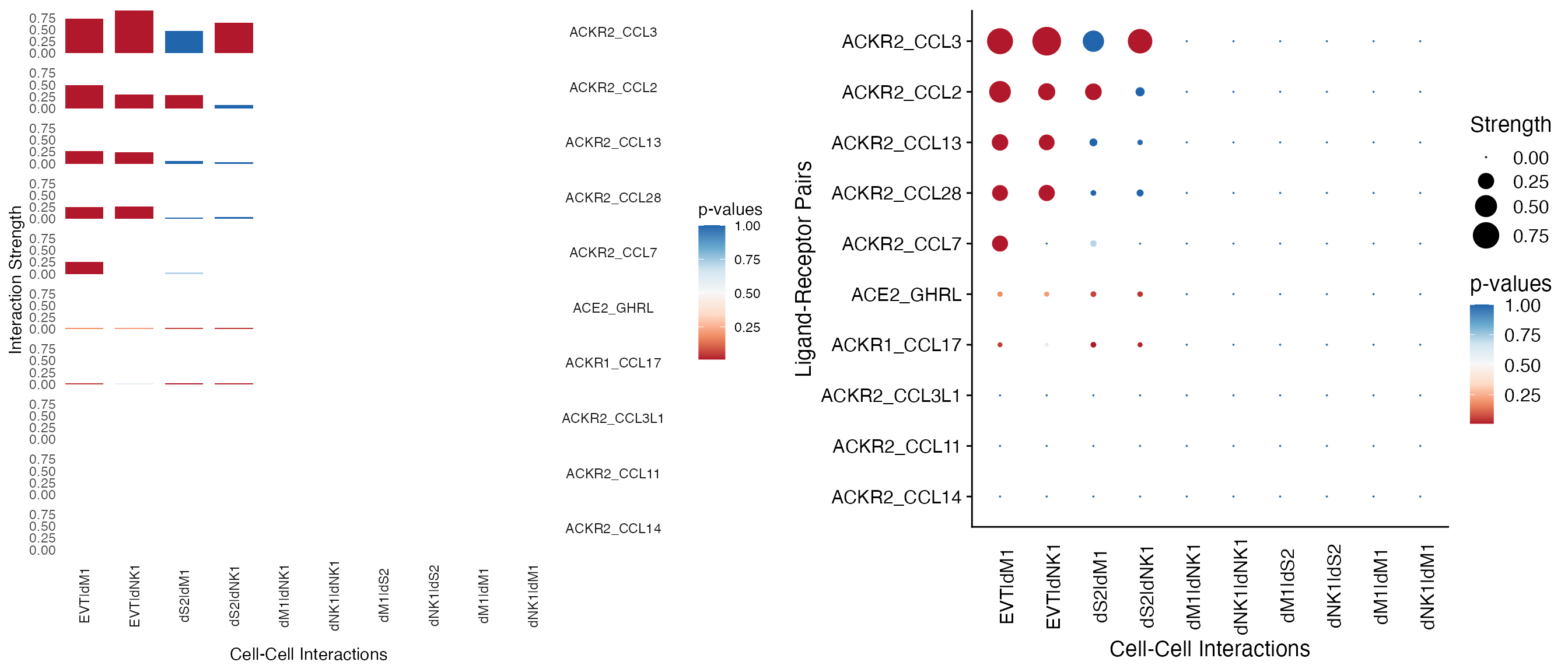

PlotHeatmap generates a heatmap. It takes arguments similar to PlotSpot. In addition, it can provide a summarized view by aggregating interaction data:
- selected use @selected data if calculated.
- aggregate type of aggregation to use. Options include cell and gene.
- counted aggregate interaction counts instead of strengths.
- scale scale and center the data to plot.
- Additional arguments see ?PlotHeatmap for details.

We use PlotHeatmap to visualize the most interactive cell types by setting aggregate = "cell".

PlotHeatmap(object = decidua.interaction.emd, aggregate = "cell", order = TRUE, selected = TRUE, mar = c(10,10))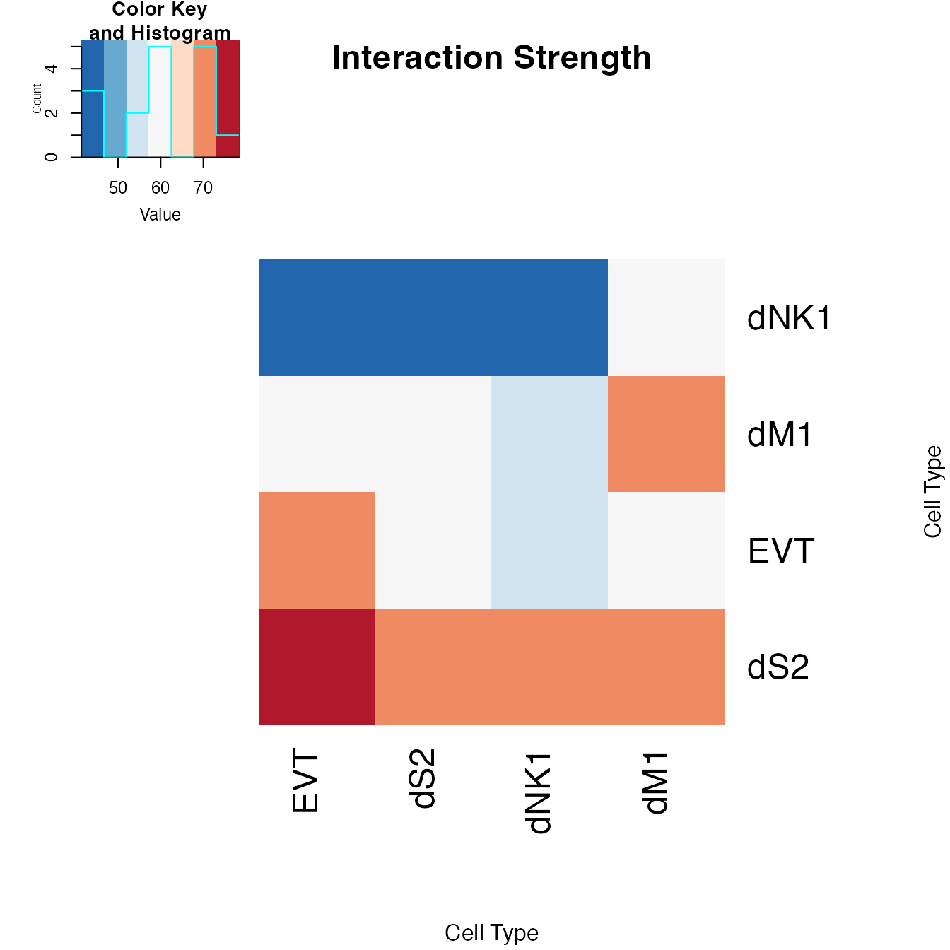

PlotNetwork generates a gene-gene or cell-cell interaction network plot. It takes arguments similar to PlotHeatmap:
- selected use @selected data if calculated.
- aggregate type of aggregation to use. Options include cell and gene.
- node.size, node.color and edge.color size and color of the nodes and edges.
- layout layout used to plot network (i.e tsne or umap layout).
- directed plots directed network.
- louvain performs louvain clustering.
- Additional arguments see ?PlotNetwork for details.

We use PlotNetwork to visualize the cell-cell interaction network by setting aggregate = "cell".

PlotNetwork(object = decidua.interaction.emd, aggregate = "cell", selected = TRUE, legend.posit = "topleft", legend.breaks = 3)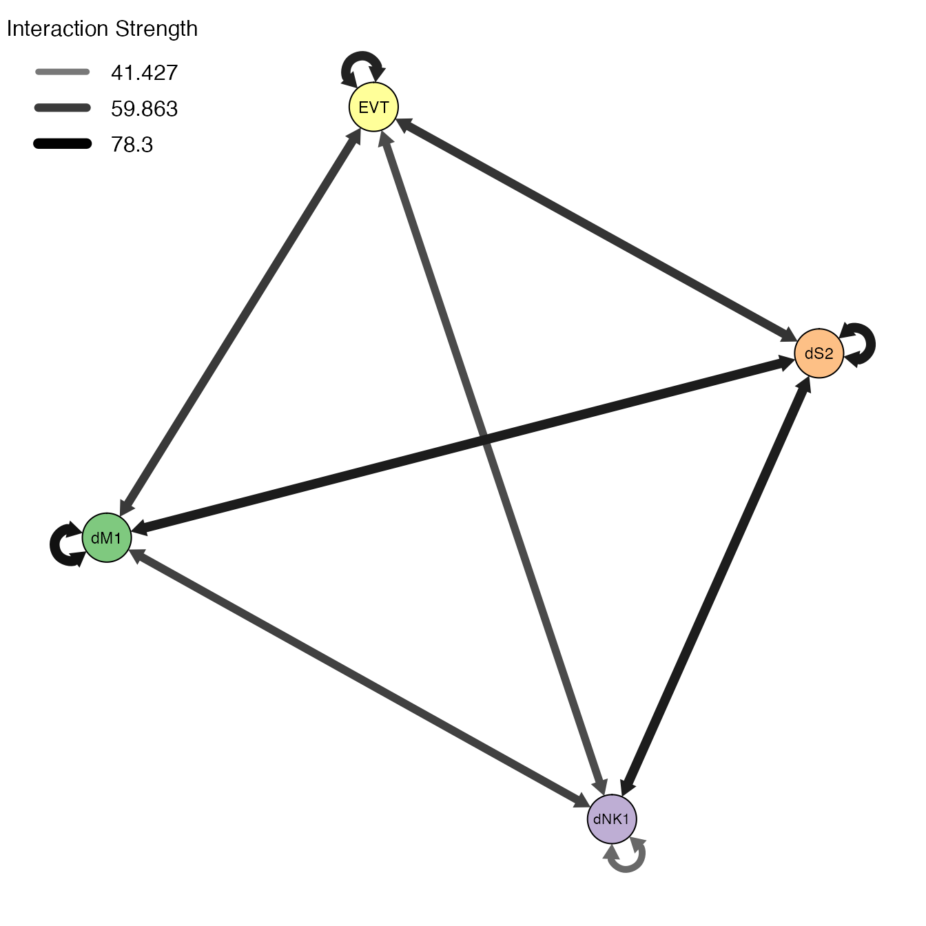

We can also use PlotNetwork to visualize the gene-gene interaction network by setting aggregate = "gene".

PlotNetwork(object = decidua.interaction.emd, aggregate = "gene", louvain = TRUE, selected = TRUE, filter = TRUE, low.cutoff = 5, node.size = 4, legend.posit = "bottomright")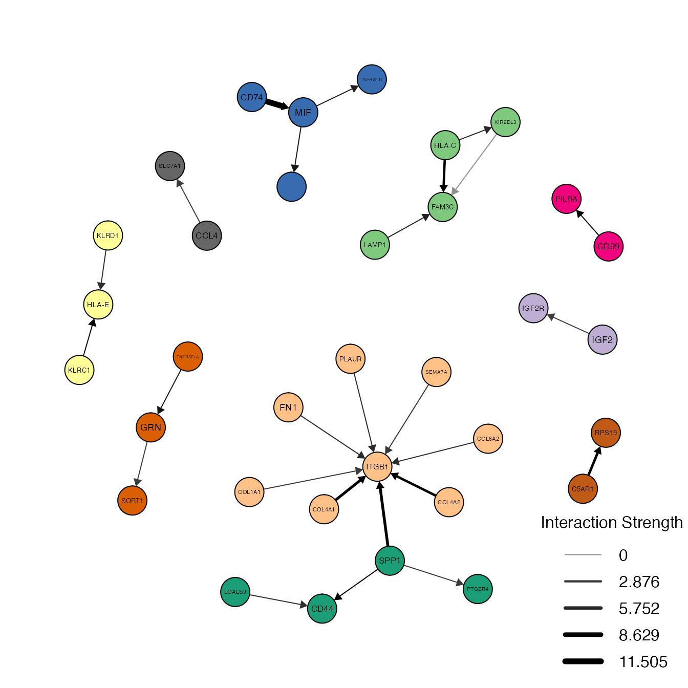

The PlotScatter function generates visualization of expression profiles for specific gene-gene interactions among all other interactions in a given pair of cell-cell interaction.

# Visualize ITGB1-PLAUR interactions between EVT and dM1 cells.
PlotScatter(object = decidua.interaction.emd, ident1 = "dM1", ident2 = "EVT", ligands = "ITGB1", receptors = "PLAUR", add.lines = TRUE, point.cex = 2)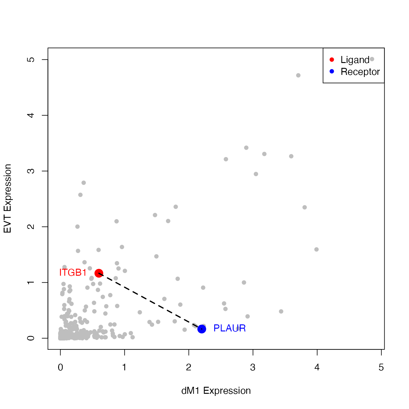

PlotHistogram generates a histogram to visualize the ligand and receptor expressions in interacting cell types. Possible arguments include:
- ligand and receptor ligand and receptor gene names.
- ligand.ident and receptor.ident Cell types to plot for ligand and receptor.
- nbins Number of bins to use for histogram.
- Additional arguments see ?PlotHistogram for details.

We use PlotHistogram to visualize the top interacting ligand-receptor pairs in the base model: CD74_MIF and CD74_APP in dM1|EVT and dM1|dS2 cell-cell interactions respectively. We can see that the base model prioritizes higher mean expression values of ligand and receptor pairs, regardless of their variable distributions.

par(mfrow = c(1,2))

# Histogram for CD74 and MIF interaction between dM1 and EVT cells.
PlotHistogram(object = decidua.interaction, ligand = "MIF", receptor = "CD74", ligand.ident = "EVT", receptor.ident = "dM1", nbins = 25)

# Histogram for CD74 and APP interaction between dM1 and dS2 cells.
PlotHistogram(object = decidua.interaction, ligand = "APP", receptor = "CD74", ligand.ident = "dS2", receptor.ident = "dM1", nbins = 25)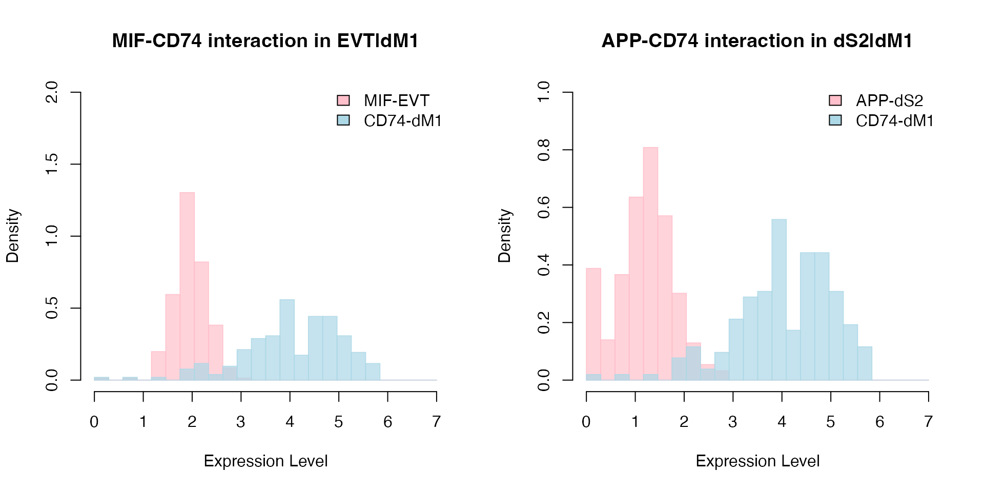

We then use PlotHistogram to visualize the top interacting ligand-receptor pairs in the EMD model: FLT1_PGF and KLRC1_HLA-E in EVT|EVT and dNK1|dM1 cell-cell interactions respectively. The results show that the EMD model takes into account the variability in the distributions between ligand and receptor pair. It is not biased towards higher mean expression values in either ligand or receptor. It selects the best "matching" pairs.

par(mfrow = c(1,2))

# Histogram for KLRC1 and HLA-E interaction between dNK1 and dM1 cells.
PlotHistogram(object = decidua.interaction.emd, ligand = "KLRC1", receptor = "HLA-E", ligand.ident = "dNK1", receptor.ident = "dM1", nbins = 25)

# Histogram for FLT1 and PGF interaction between EVT and EVT cells.
PlotHistogram(object = decidua.interaction.emd, ligand = "PGF", receptor = "FLT1", ligand.ident = "EVT", receptor.ident = "EVT", nbins = 25)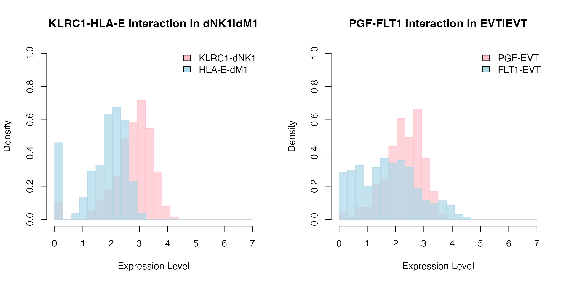

Lastly, we compare the base model (x axis) against the EMD model (y axis). We see that the baseline model creates quite a few false-positives (dark red dots in lower right).

plot(x = decidua.interaction@strength, 
     y = decidua.interaction.emd@strength, 
     xlab = "Base Model", ylab = "EMD Adjusted", 
     col = RColorBrewer::brewer.pal(5,"Reds")[cut(decidua.interaction@strength-decidua.interaction.emd@strength,5)],
     pch = 16)
abline(-0.2, 1, col = "red", lwd = 2, lty = 2)
abline(0.1, 1, col = "red", lwd = 2,lty = 2)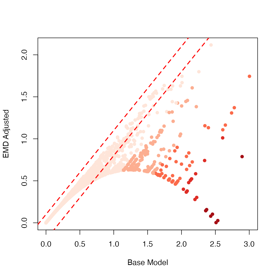

# R session information.
sessionInfo()
## R version 4.0.3 (2020-10-10)
## Platform: x86_64-apple-darwin17.0 (64-bit)
## Running under: macOS Big Sur 10.16
## 
## Matrix products: default
## BLAS:   /Library/Frameworks/R.framework/Versions/4.0/Resources/lib/libRblas.dylib
## LAPACK: /Library/Frameworks/R.framework/Versions/4.0/Resources/lib/libRlapack.dylib
## 
## locale:
## [1] en_US.UTF-8/en_US.UTF-8/en_US.UTF-8/C/en_US.UTF-8/en_US.UTF-8
## 
## attached base packages:
## [1] stats     graphics  grDevices utils     datasets  methods   base     
## 
## other attached packages:
## [1] scMatchmaker_0.99.0
## 
## loaded via a namespace (and not attached):
##   [1] nlme_3.1-151        bitops_1.0-6        matrixStats_0.57.0  fs_1.5.0            doParallel_1.0.16   RColorBrewer_1.1-2  rprojroot_2.0.2    
##   [8] tools_4.0.3         backports_1.2.1     bslib_0.3.1         R6_2.5.0            irlba_2.3.3         d3Network_0.5.2.1   rpart_4.1-15       
##  [15] KernSmooth_2.23-18  Hmisc_4.4-2         colorspace_2.0-0    nnet_7.3-14         tidyselect_1.1.0    gridExtra_2.3       mnormt_2.0.2       
##  [22] compiler_4.0.3      qgraph_1.6.5        fdrtool_1.2.16      textshaping_0.2.1   cli_3.2.0           htmlTable_2.1.0     TSP_1.1-10         
##  [29] desc_1.4.1          labeling_0.4.2      sass_0.4.0          caTools_1.18.0      scales_1.1.1        checkmate_2.0.0     psych_2.0.12       
##  [36] pbapply_1.4-3       pkgdown_2.0.2       pbivnorm_0.6.0      systemfonts_0.3.2   stringr_1.4.0       digest_0.6.27       foreign_0.8-81     
##  [43] rmarkdown_2.13      base64enc_0.1-3     jpeg_0.1-8.1        pkgconfig_2.0.3     htmltools_0.5.2     highr_0.8           fastmap_1.1.0      
##  [50] htmlwidgets_1.5.3   rlang_1.0.2         huge_1.3.4.1        rstudioapi_0.13     farver_2.0.3        jquerylib_0.1.3     generics_0.1.0     
##  [57] jsonlite_1.7.2      gtools_3.8.2        dplyr_1.0.2         magrittr_2.0.1      Formula_1.2-4       Matrix_1.3-2        Rcpp_1.0.7         
##  [64] munsell_0.5.0       reticulate_1.18     abind_1.4-5         lifecycle_1.0.1     whisker_0.4         stringi_1.5.3       yaml_2.2.1         
##  [71] MASS_7.3-53         gplots_3.1.1        plyr_1.8.6          lavaan_0.6-7        grid_4.0.3          parallel_4.0.3      crayon_1.3.4       
##  [78] lattice_0.20-41     cowplot_1.1.1       splines_4.0.3       tmvnsim_1.0-2       knitr_1.38          pillar_1.4.7        igraph_1.2.6       
##  [85] rjson_0.2.20        corpcor_1.6.9       BDgraph_2.63        stats4_4.0.3        reshape2_1.4.4      codetools_0.2-18    glue_1.6.2         
##  [92] evaluate_0.15       emdist_0.3-1        latticeExtra_0.6-29 data.table_1.13.6   png_0.1-7           vctrs_0.4.1         foreach_1.5.1      
##  [99] gtable_0.3.0        purrr_0.3.4         cachem_1.0.1        ggplot2_3.3.3       xfun_0.30           glasso_1.11         ragg_0.4.0         
## [106] survival_3.2-7      seriation_1.2-9     tibble_3.0.4        iterators_1.0.13    registry_0.5-1      memoise_2.0.1       cluster_2.1.0      
## [113] ellipsis_0.3.2

Last Run: May 14, 2022

Setup the Matchmaker Object

Identify Cell-Cell Interactions with Matchmaking

Select Top Interactions

Visualize Cell-Cell Interactions